To tylko jedna z 5 stron tej notatki. Zaloguj się aby zobaczyć ten dokument.
Zobacz
całą notatkę
Measurement and modeling
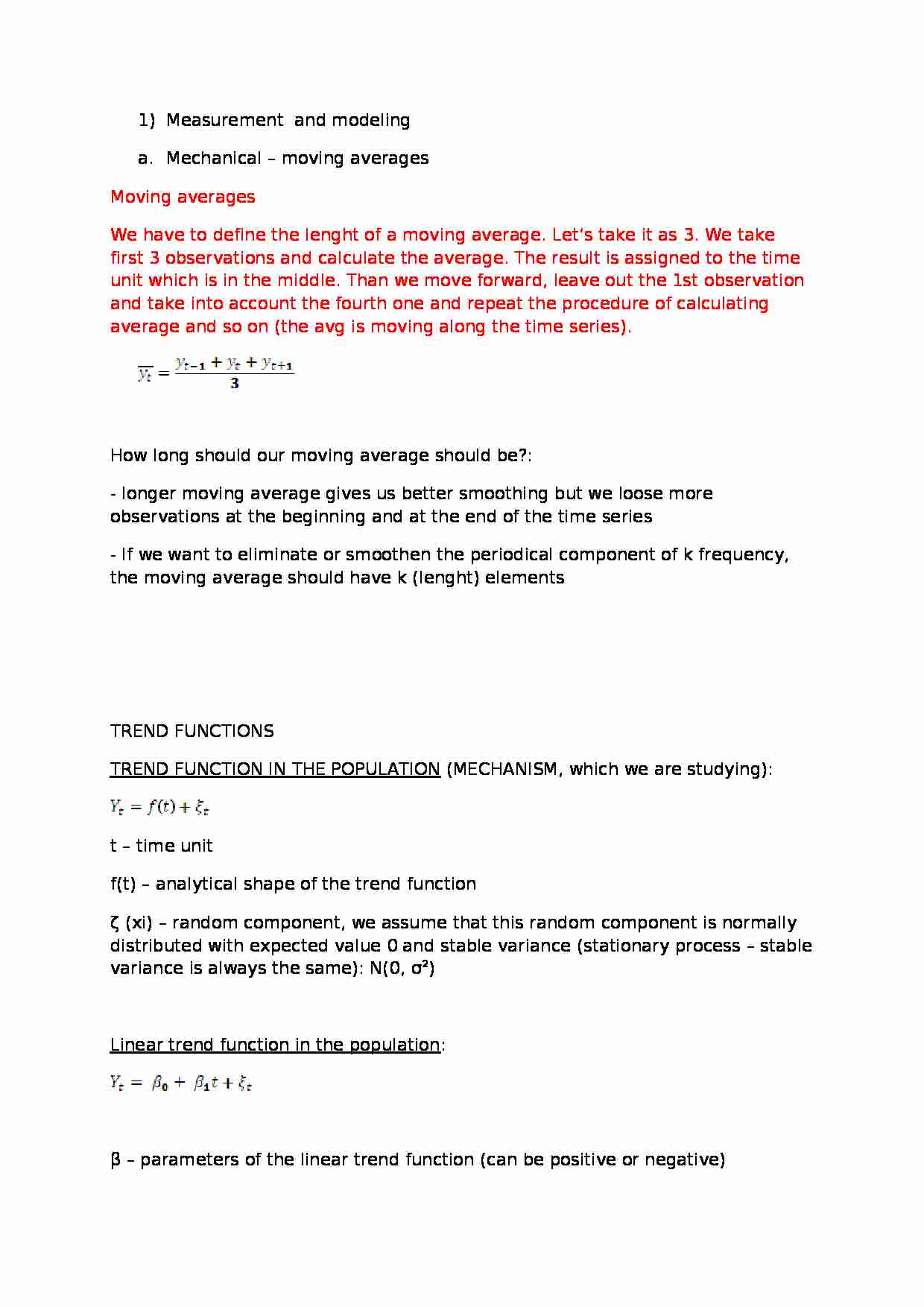
Mechanical - moving averages Moving averages We have to define the lenght of a moving average. Let's take it as 3. We take first 3 observations and calculate the average. The result is assigned to the time unit which is in the middle. Than we move forward, leave out the 1st observation and take into account the fourth one and repeat the procedure of calculating average and so on (the avg is moving along the time series). How long should our moving average should be?:
- longer moving average gives us better smoothing but we loose more observations at the beginning and at the end of the time series
- If we want to eliminate or smoothen the periodical component of k frequency, the moving average should have k (lenght) elements TREND FUNCTIONS
TREND FUNCTION IN THE POPULATION (MECHANISM, which we are studying):
t - time unit
f(t) - analytical shape of the trend function
ζ (xi) - random component, we assume that this random component is normally distributed with expected value 0 and stable variance (stationary process - stable variance is always the same): N(0, σ 2 )
Linear trend function in the population :
β - parameters of the linear trend function (can be positive or negative)
β 0 - intercept (the place in which trend function crosses OY axis (vertical axis), or this is the average level of Y in t=0 (time unit number by0)
β 1 - slope - the average change of Y in 1 time unit (in our case the average yearly change)
We estaimate trend parameter with OLS (Ordinary Least Squares) method.
Linear trend sample (our time series) in the population: y t - observed values of variable y
t - time variable
b 0 - estimator of β 0 : sample intercept
b 1 - estimator of β 1 : sample slope (sometimes called trend coeficient)
ε t - residuals (reszty) or error term, observed values of random component ζ (xi)
- ( y hat ) - theoretical value of a trend function (value calculated from the model)
There are two general types of time series:
Additive - Y = trend + seasonality + error
Multiplicative - Y = trend*seasonality*error
Generally we have 2 seasonal models:
Additive - Y=trend+seasonality+randomness - it's wehen diviations from the trend are of the same level no matter where we r on our time series.
Multiplicative - Y=trend + Seasonality - deviations from the trend r becoming bigger while trend line is going up.
One of the time variables is statistically significant - all p-values for them are bigger than significance level (0.05). It means that the order of my polynomial is too high. On the other hand, according to backward stepwise-regression rule we should eliminate that variable, which has the highest p-value. Both criteria say that t
... zobacz całą notatkę
Komentarze użytkowników (0)