To tylko jedna z 17 stron tej notatki. Zaloguj się aby zobaczyć ten dokument.
Zobacz
całą notatkę
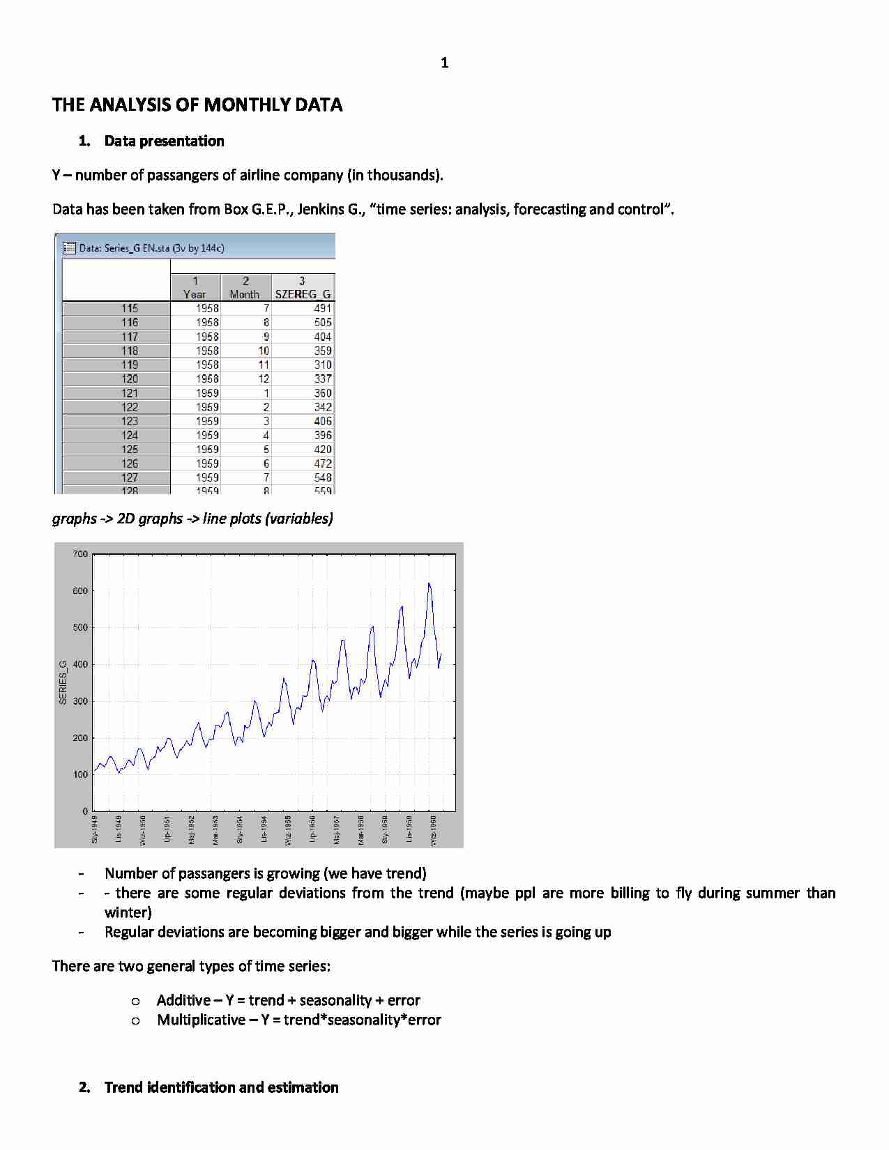
THE ANALYSIS OF MONTHLY DATA Data presentation Y - number of passangers of airline company (in thousands).
Data has been taken from Box G.E.P., Jenkins G., “time series: analysis, forecasting and control”.
graphs - 2D graphs - line plots (variables) Number of passangers is growing (we have trend)
- there are some regular deviations from the trend (maybe ppl are more billing to fly during summer than winter)
Regular deviations are becoming bigger and bigger while the series is going up
There are two general types of time series:
Additive - Y = trend + seasonality + error
Multiplicative - Y = trend*seasonality*error
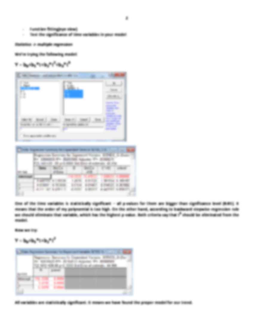
Trend identification and estimation Function fitting(eye view)
Test the significance of time variables in your model Statistics - multiple regression We're trying the following model:
Y = b 0 +b 1 *t+b 2 *t 2 +b 3 *t 3 One of the time variables is statistically significant - all p-values for them are bigger than significance level (0.05). It means that the order of my polynomial is too high. On the other hand, according to backward stepwise-regression rule we should eliminate that variable, which has the highest p-value. Both criteria say that t 3 should be eliminated from the model.
Now we try:
Y = b 0 +b 1 *t+b 2 *t 2 All variables are statistically significant. It means we have found the proper model for our trend.
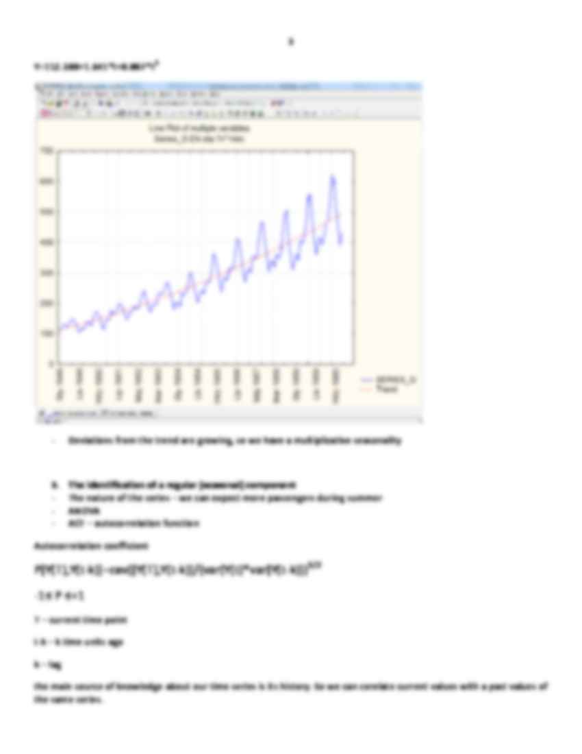
Y=112.380+1.641*t+0.007*t 2 Deviations from the trend are growing, so we have a multiplicative seasonality The identification of a regular (seasonal) component The nature of the series - we can expect more passengers during summer
ANOVA
ACF - autocorrelation function
Autocorrelation coefficient
Ρ[Y(T),Y(t-k)]=cov([Y(T),Y(t-k)]/{var(Y(t)*var[Y(t-k)]} 1/2 -1≤ Ρ ≤+1
T - current time point
t-k - k time units ago
k - lag
the main source of knowledge about our time series is its history. So we can corelate current values with a past values of the same series.
If autocorrelation coefficients depend only on k, but not on t - then we can have Autocorrelation function:
-1≤ Ρ k ≤+1
Autocorrelation function should be calculated only from detrended data. So we should eliminate the trend first.
22.05
The estimation of ACF (autocorrelation function)
Advanced linear/nonlinear models - time series forcasting.
Some useful transformations
Logarithm - using this transformation u can stabilise variance (variability) when arience is becoming bigger while series is going up.
... zobacz całą notatkę
Komentarze użytkowników (0)